Step-by-Step Guide to Normal, Binomial, and Poisson Distributions Using Python

 Understanding probability distributions is essential for anyone working in data science, statistics, or machine learning.

In this blog, we’ll break down three of the most common distributions — Normal, Binomial, and Poisson — along with easy-to-follow Python examples using real-world data.

Whether you’re building a predictive model or analyzing data patterns, mastering these distributions will sharpen your skills.

Let’s dive in!

What Are Probability Distributions?

A probability distribution describes how the values of a random variable are distributed.

It tells you the probability of different outcomes — kind of like a weather report, but for data!

There are two broad types:

• Discrete distributions: Deal with countable outcomes (e.g., number of cars).
• Continuous distributions: Deal with outcomes that can take any value within a range (e.g., height, weight).

1. Normal Distribution — The Bell Curve Superstar

What is it?

The Normal distribution is a continuous distribution that is symmetric around the mean.

Most natural phenomena (like heights, blood pressure, or IQ scores) follow this distribution.

Formula:

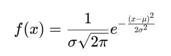
Where:

• μ = Mean (center of the distribution)
• σ = Standard deviation (spread of the distribution)
• x = Value of the random variable

Python Implementation using Seaborn’s mpg Dataset

We’ll explore the mpg (miles per gallon) distribution using seaborn's built-in dataset.

import seaborn as sns
import matplotlib.pyplot as plt
from scipy.stats import norm

# Generate Normal Distribution (Titanic 'age' data)
titanic = sns.load_dataset('titanic')
age_data = titanic['age'].dropna()

# Plot
sns.histplot(age_data, kde=True)
plt.title('Age Distribution (Normal Approximation)')
plt.xlabel('Age')
plt.ylabel('Density')
plt.show()

Output:

Statistical Test: Checking Normality (Shapiro-Wilk Test)

Before assuming the data is normally distributed based on looks, let’s test it properly.

The Shapiro-Wilk Test checks whether a sample comes from a normal distribution.

• Null Hypothesis (H₀): Data is normally distributed.
• Alternative Hypothesis (H₁): Data is not normally distributed.

from scipy.stats import shapiro

# Shapiro-Wilk test
stat, p_value = shapiro(age_data)
print(f"Shapiro-Wilk Test p-value: {p_value:.4f}")

if p_value > 0.05:
    print("Data is likely normally distributed.")
else:
    print("Data is likely NOT normally distributed.")

Interpretation:

• If p-value > 0.05, we fail to reject H₀: data is likely normal.
• If p-value ≤ 0.05, we reject H₀: data is not normal.

Output:

Shapiro-Wilk Test p-value: 0.0000
Data is likely NOT normally distributed.

Since the p-value is less than 0.05, we conclude that the `age` variable is not perfectly normal.

(But it still looks close enough for practical purposes in many cases.)

2. Binomial Distribution — Success or Failure?

What is it?

The Binomial distribution is a discrete distribution. It describes the number of successes in a fixed number of independent yes/no experiments.

Think coin tosses, exam passes, or product clicks!

Formula:

Where:

• n = number of trials
• p = probability of success in a single trial
• k = number of successes
• (n k) = number of ways to choose k successes from n trials

Practical Example: Email Campaign Success

Suppose you’re running an email marketing campaign. You send emails to 10 customers and based on past experience, you know that 20% of them typically click on the link.

What’s the probability that exactly 2 customers click the link?

from scipy.stats import binom

# Parameters
n = 10  # Number of customers emailed
p = 0.2  # Probability of a customer clicking the link
k = 2  # Number of clicks

# Probability Mass Function
prob = binom.pmf(k, n, p)
print(f"Probability that exactly 2 customers click the link: {prob:.2f}")

Output:

Probability that exactly 2 customers click the link: 0.30

So there’s roughly a 30% chance that exactly 2 customers out of 10 will click on the link.

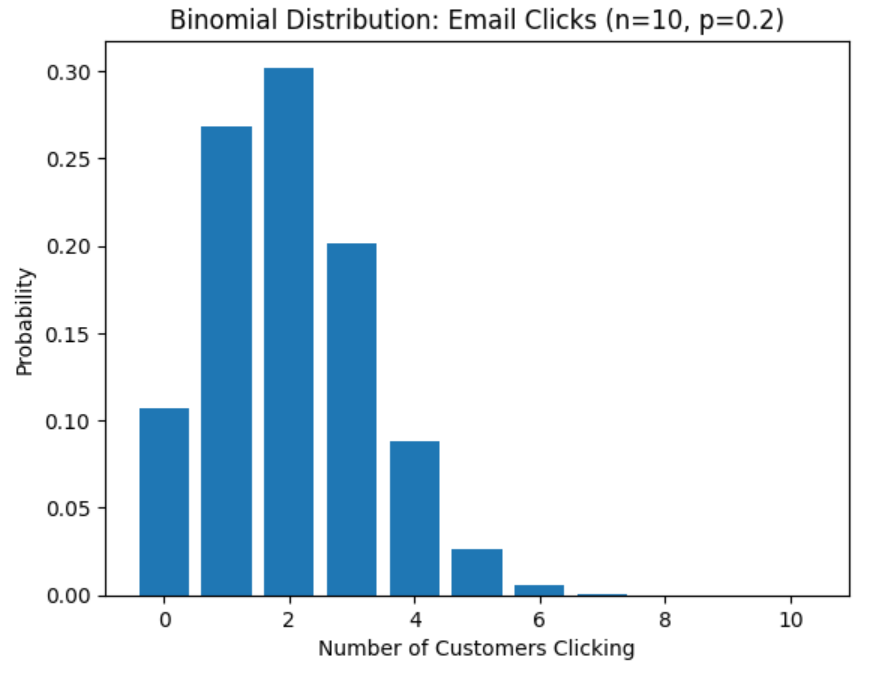
Bonus: Visualizing the Email Clicks Distribution

import numpy as np
x = np.arange(0, n+1)
y = binom.pmf(x, n, p)
plt.bar(x, y)
plt.title('Binomial Distribution: Email Clicks (n=10, p=0.2)')
plt.xlabel('Number of Customers Clicking')
plt.ylabel('Probability')
plt.show()

Output:
A bar plot showing the probability of 0, 1, 2, …, 10 customers clicking the email link. You’ll notice that 2 or 3 clicks are the most probable outcomes — matching marketing intuition!

3. Poisson Distribution — Counting Events

What is it?

The Poisson distribution models the number of times an event occurs in a fixed interval of time or space, assuming events happen independently and at a constant average rate.

Examples include:

• Number of emails received per hour
• Number of cars passing a checkpoint

Formula:

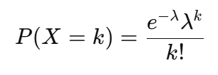
Where:

• λ = Average number of occurrences (mean)
• k = Number of occurrences
• e = Euler’s number (~2.718)

Python Implementation: Restaurant Orders Example

Suppose a restaurant receives 4 orders per minute. What’s the probability they receive 2 orders in the next minute?

from scipy.stats import poisson

# Parameters
lambda_ = 4  # Average orders per minute
k = 2  # Actual number of orders

# Probability
prob = poisson.pmf(k, mu=lambda_)
print(f"Probability of receiving exactly 2 orders: {prob:.2f}")

Output:

Probability of receiving exactly 2 orders: 0.15

Bonus Visualization: Poisson Distribution Plot

x = np.arange(0, 10)
y = poisson.pmf(x, mu=lambda_)
plt.bar(x, y)
plt.title('Poisson Distribution (λ=4)')
plt.xlabel('Number of Orders')
plt.ylabel('Probability')
plt.show()

Output:
 A bar plot showing probabilities for receiving 0 to 9 orders.

Quick Summary Table

To conclude:

Mastering Normal, Binomial, and Poisson distributions is crucial for any aspiring data analyst, statistician, or machine learning engineer.

These distributions help you model the real world more accurately, choose the right algorithms, and make smarter predictions.

Use statistical tests like the Shapiro-Wilk test to check assumptions rather than just trusting your plots.

And remember:

Data without distributions is like pizza without cheese — still edible, but not nearly as good!

If you learned anything new from this blog, then request you to please hit that clap button and share it with someone who’s interested in Statistics, Probability Distributions, and Data science!

If you’re as passionate about AI, ML, DS, Strategy and Business Planning as I am, I invite you to:
Connect with me:

• On LinkedIn.

• Career Counselling and Mentorship: Topmate

• Join my Whatsapp Group where I share resources, links, and updates.

Happy Learning!