A Step-by-Step Tutorial
Decision trees are easy to understand and interpret but can easily overfit, especially on imbalanced datasets. So, in this guide, we’ll work through building a Decision Tree Classifier on an imbalanced dataset, evaluate its performance, perform hyperparameter tuning, and even plot the decision tree.

What is a Decision Tree?
A Decision Tree is a supervised machine learning algorithm used for both classification and regression tasks. It works by splitting the data into different subsets based on the most significant features (decisions), forming a tree structure. At each node, the algorithm asks a yes/no question, and branches are formed based on the answer.
Build a Decision Tree Classifier on an Imbalanced Dataset
Let’s dive into the practical implementation by creating an imbalanced dataset and building a decision tree.
Step 1: Create an Imbalanced Dataset
We’ll create a dataset where 95% of the target class belongs to `0` and only 5% belongs to the positive class `1`.
from sklearn.datasets import make_classification
import pandas as pd

# Create a synthetic imbalanced dataset with 1000 samples, 10 features, and 5% positive class
X, y = make_classification(n_samples=1000, n_features=10, n_classes=2,
                           weights=[0.95, 0.05], random_state=42)

# Convert to DataFrame for easy manipulation
data = pd.DataFrame(X, columns=[f'Feature_{i}' for i in range(1, 11)])
data['Target'] = y

data.head()
Output:

This dataset simulates an imbalanced classification problem, where we have ten features and one target variable.
The distribution of target variable indicates that only 5% of the data belongs to the positive class (`1`).
# Show the class distribution
print(data['Target'].value_counts(normalize=True))
Output:

Step 2: Train-Test Split
The next step is to split the data into training (70%) and testing (30%) sets.
from sklearn.model_selection import train_test_split

# Separate features and target
X = data.drop(columns=['Target'])
y = data['Target']

# Split the dataset into training and testing sets (70% train, 30% test)
X_train, X_test, y_train, y_test = train_test_split(X, y, test_size=0.3, random_state=42, stratify=y)
The stratify=yensures the training and testing sets maintain the original imbalance in the target class.
Step 3: Build the Decision Tree Classifier
Since we have an imbalanced dataset, we will use `class_weight=’balanced’` parameter to address the imbalance during training.
from sklearn.tree import DecisionTreeClassifier

# Initialize the Decision Tree Classifier with class weight balanced
dt_classifier = DecisionTreeClassifier(random_state=42, class_weight='balanced')

# Train the model
dt_classifier.fit(X_train, y_train)
Step 4: Evaluate the Model Performance
The next step is to evaluate the model performance on the train and test sets using metrics like the confusion matrix, F1-score, and AUC score to get a comprehensive understanding of how well the model performs, especially on the minority class.
The code below provides performance metrics for both the training and test sets, allowing us to see how well the decision tree handles the imbalanced data.
from sklearn.metrics import classification_report, confusion_matrix, roc_auc_score

# Predictions on train and test sets
y_train_pred = dt_classifier.predict(X_train)
y_test_pred = dt_classifier.predict(X_test)

# Confusion Matrix, Classification Report, and AUC score for Training Set
print("Training Set:")
print(confusion_matrix(y_train, y_train_pred))
print(classification_report(y_train, y_train_pred))
train_auc = roc_auc_score(y_train, dt_classifier.predict_proba(X_train)[:, 1])
print("AUC Score (Train):", train_auc)

# Confusion Matrix, Classification Report, and AUC score for Testing Set
print("\nTesting Set:")
print(confusion_matrix(y_test, y_test_pred))
print(classification_report(y_test, y_test_pred))
test_auc = roc_auc_score(y_test, dt_classifier.predict_proba(X_test)[:, 1])
print("AUC Score (Test):", test_auc)
Output:

You can see that the model performs perfectly well on the training set, but its performance (recall parameter) goes down on the test set, especially for the positive class, which is the minority class.
Visualize the Most Important Features
One of the important considerations in a machine learning modelling process is to understand the most significant predictors. If we can visualize the same, that’s even better.
Decision trees allow us to calculate and visualize feature importance based on how much a feature contributes to reducing impurity at each split. Let’s visualize the feature importance in descending order with the code below.
import matplotlib.pyplot as plt
import numpy as np

# Get feature importances from the model
importances = dt_classifier.feature_importances_
features = X.columns

# Sort features by importance in descending order
indices = np.argsort(importances)[::-1]

# Plot the feature importances in descending order
plt.figure(figsize=(10,6))
plt.title("Feature Importance (Sorted) - Decision Tree")
plt.barh(range(len(indices)), importances[indices], align='center')
plt.yticks(range(len(indices)), [features[i] for i in indices])
plt.xlabel('Relative Importance')
plt.gca().invert_yaxis()  # To have the most important feature at the top
plt.show()
This will give a bar chart showing which features were most influential in the model’s decision-making process.

Hyperparameter Tuning with GridSearchCV
Tuning hyperparameters can significantly improve the performance of a decision tree.
Here are some of the key hyperparameters that are considered while building a decision tree:
- `max_depth`: Controls the maximum depth of the tree. Deep trees may overfit, so tuning this value can reduce overfitting.
- `min_samples_split`: The minimum number of samples required to split an internal node. Increasing this helps prevent small, noisy splits.
- `min_samples_leaf`: The minimum number of samples that a leaf node can have. Increasing this value reduces overfitting.
- `class_weight`: Useful for handling imbalanced data by giving more weight to the minority class.
Let’s tune the decision tree’s hyperparameters using `GridSearchCV`. We’ll optimize some of the parameters discussed above.
from sklearn.model_selection import GridSearchCV

# Define the parameter grid
param_grid = {
    'max_depth': [3, 6, 10],
    'min_samples_split': [2, 5, 10],
    'min_samples_leaf': [1, 2, 4]
}

# Initialize GridSearchCV
grid_search = GridSearchCV(estimator=dt_classifier, param_grid=param_grid,
                           cv=3, n_jobs=-1, scoring='roc_auc')

# Fit the grid search model
grid_search.fit(X_train, y_train)

# Best parameters from the search
print("Best Parameters:", grid_search.best_params_)
Output:

So we have got the best hyperparameters basis the grid search we did. After finding the best hyperparameters, we can retrain the decision tree with these optimized values and re-evaluate it.
Evaluate the Optimized Model
Let’s evaluate the optimized model with the code below.
# Initialize the Decision Tree Classifier with optimized parameters
dt_classifier_optimized = grid_search.best_estimator_

# Train the optimized model
dt_classifier_optimized.fit(X_train, y_train)

# Evaluate the optimized model
y_train_pred_optimized = dt_classifier_optimized.predict(X_train)
y_test_pred_optimized = dt_classifier_optimized.predict(X_test)

# Confusion Matrix and AUC for the optimized model - Training Set
print("Optimized Training Set:")
print(confusion_matrix(y_train, y_train_pred_optimized))
print(classification_report(y_train, y_train_pred_optimized))
train_auc_optimized = roc_auc_score(y_train, dt_classifier_optimized.predict_proba(X_train)[:, 1])
print("AUC Score (Train - Optimized):", train_auc_optimized)

# Confusion Matrix and AUC for the optimized model - Testing Set
print("\nOptimized Testing Set:")
print(confusion_matrix(y_test, y_test_pred_optimized))
print(classification_report(y_test, y_test_pred_optimized))
test_auc_optimized = roc_auc_score(y_test, dt_classifier_optimized.predict_proba(X_test)[:, 1])
print("AUC Score (Test - Optimized):", test_auc_optimized)
Output:

You can see that the performance of the optimized model in terms of recall is almost same as the earlier version of the model. This can be improved by giving a much wider range to grid search options, however remember that it will increase the computational load on model training.
Something you can try out at your end!
Plot the Optimized Decision Tree
Finally, let’s visualize the final, optimized decision tree using `plot_tree` from `sklearn`.
from sklearn.tree import plot_tree
import matplotlib.pyplot as plt

# Set up the plot size
plt.figure(figsize=(20,10))

# Plot the optimized decision tree
# Plot the optimized decision tree
plot_tree(dt_classifier_optimized, feature_names=X.columns, class_names=['Class 0', 'Class 1'],
          filled=True, rounded=True, fontsize=10)

# Show the plot
plt.show()
Output:
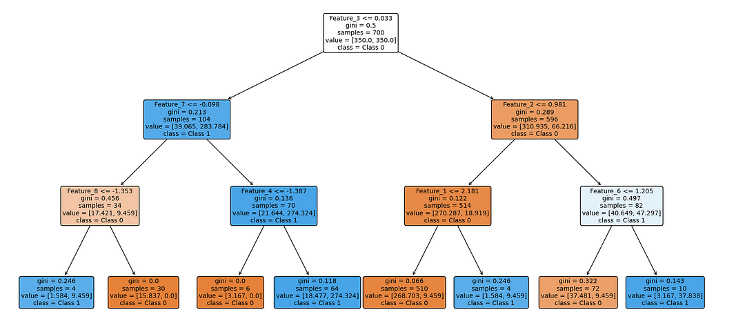
The plot above will give a visual representation of the optimized decision tree, showing how it splits the data based on the most important features.
Final Thoughts
In this tutorial, we explored the Decision Tree Classifier in Python, focusing on building the model with an imbalanced dataset.
We covered the following:
1. Decision tree basics: How decision trees work and why they are useful.
2. Imbalanced data: We created an imbalanced dataset to simulate a real-world scenario.
3. Model evaluation: We used key metrics like the confusion matrix, F1-score, and AUC score to evaluate model performance.
4. Feature importance: We visualized the most important features used by the decision tree.
5. Hyperparameter tuning: We optimized the decision tree using `GridSearchCV` to improve performance.
6. Tree visualization: We visualized the final decision tree to better understand how the model makes decisions.
Next Steps
Decision trees are powerful but prone to overfitting, especially with imbalanced datasets. Now that you’ve built and tuned a decision tree, you can experiment with different datasets and further tune hyperparameters to get the best results. You can also explore ensemble methods like Random Forest or Bagging to boost performance, something we’ll cover in the future guides.
Happy coding, and enjoy your machine learning journey! 😊
- On LinkedIn.
- Career Counselling and Mentorship: Topmate
- Join my Whatsapp Group where I share resources, links, and updates.
Comments
Post a Comment